Pre-tender turbidity assessment

To evaluate the potential impact of dredging near the seawater intake facility, Sohar Port, in collaboration with a specialised consultant, conducted an early pre-tender turbidity assessment. The aim was to determine the sensitivity of the intake to the turbidity generated by on-site dredging operations. This step was critical to demonstrate the feasibility of dredging near the seawater intake. It also provided a foundation for open discussions with relevant stakeholders regarding realistic turbidity limits to be included in the required permits and No Objection Certificates (NOCs).

The objectives of the turbidity modeling study were as follows:

• To determine the extent of fine sediment plumes resulting from dredging activities;
• To assess the increase in suspended sediment concentrations above ambient levels caused by dredging operations; and
• To propose mitigation measures to minimise the impact of fine sediment plumes generated during the works.

At the time of the study, the exact details of how the dredging operations would be carried out were not yet determined. A conservative but realistic approach was taken, as described in the following section.

Model approach and input parameters

A detailed Delft3D-FLOW (http://oss. deltares.nl/web/delft3d/home) model was used to simulate the far-field dispersion of sediment spills resulting from dredging operations. The main location of interest for the computed suspended sediment concentration is directly in front of the pumping station, which is a sheltered area within the breakwaters of the seawater intake. This was considered the critical point, as from here the water flows into the pipeline system and is distributed to industrial users. Various exploratory dredging scenarios were developed and assessed, starting with conservative assumptions of high spill rates and continuous discharges. Based on the outcomes of these initial scenarios, more realistic scenarios were defined, incorporating a typical dredging cycle of a trailing suction hopper dredger (TSHD) and its accompanying overflow spills. Additionally, a scenario without overflow was considered, representing an adaptive dredging method that the dredging contractor could implement if necessary.

The simulations were run over a one-month period, factoring in 16 different relevant ambient wind conditions. The model also incorporated the operation of the seawater intake and outfall to ensure an accurate representation of the ambient flow conditions, including thermal effluent dispersion. All model scenarios included a weekly-averaged intake and outfall discharge of 540,000 cubic metres per hour (m³/h).

The pre-tender turbidity model only calculates the excess turbidity caused by sediment spills from the dredging operation, excluding background turbidity. For each scenario, the sediment concentrations at the intake location were converted to turbidity, measured in nephelometric turbidity units (NTU). There is no generic relationship between in-situ turbidity (NTU) and suspended sediment concentration (SSC), as computed by the model. This conversion depends on the type and size of sediment particles and is site- specific. The conversion factor was derived from a site-specific laboratory experiment that established the relationship between suspended sediment concentrations (milligrams per litre (mg/l)) and NTU turbidity levels by analysing soil bottom samples collected in the dredging footprint in combination with samples of seawater.

Fine sediment composition

The spills as fine sediment (4 micrometre (µm) to 63µm) are represented by three characteristic fine sediment fractions: 10µm, 20µm and 50µm, each with its associated fall velocities. These fractions illustrate an average distribution of 45%, 20% and 35% of the spill composition, based on data from geotechnical factual investigations conducted by a specialised geotechnical investigation company. The schematisation with three fractions is based on optimising computational efficiency while maintaining a sufficiently accurate representation of sediment dynamics, thereby avoiding the complexities that can arise from overly detailed modelling.

Modelled ambient wind conditions

Wind is a key factor in the coastal areas of Oman and plays a crucial role in the turbidity model. The region’s wind climate is characterised by a combination of land-sea breezes (LSB), low wind speeds, storms/cyclones and more persistent wind events that can last for extended periods. Wind was analysed based on long-term Climate Forecast System Reanalysis wind data. The typical ambient wind conditions throughout the year were modelled in 16 one-month scenarios (eight for summer and eight for winter), accounting for the frequency of different wind conditions in each season to ensure the scenarios collectively represent the annual wind pattern. In each modelling simulation, the wind condition remained constant throughout the computation.

Dredging scenarios considered

To assess the sensitivity of the seawater intake to the turbidity generated by the dredging activities on site above the natural background levels the following dredging scenarios were considered:

• Scenario A – typical TSHD operation with overflow, considering a dredging cycle of 2 hours and 45 minutes (min), including 90 min loading with 60 min overflow. Conservative values were applied for the drag head and overflow spill rate, respectively 10 kilograms per second (kg/ sec) and 300 kg/sec.
• Scenario B – typical TSHD operation with overflow equal to Scenario A, but additionally, a standing silt screen was considered in the model.
• Scenario C – continuous operation (no dredging cycle implemented) of TSHD without overflow and cutter suction dredger (CSD). This dredging scenario represents an alternative temporary dredging method that could be applied as part of an adaptive dredging approach when required.

Results: turbidity assessment and permit acquisition

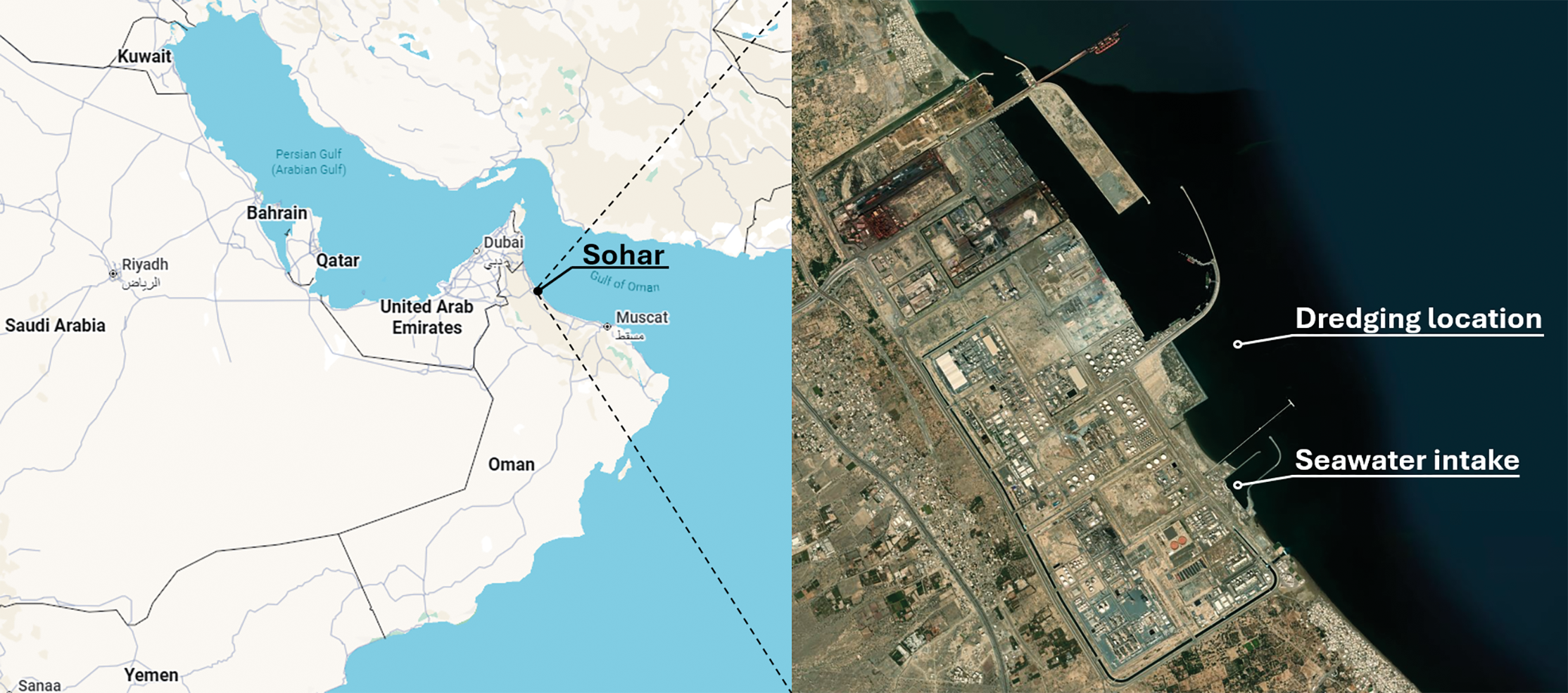
The pre-tender modelling was conducted as a feasibility assessment. Based on this initial modelling, it was concluded that dredging near the seawater intake would be feasible for all considered wind and tide conditions, provided that only the excess sediment concentrations from the dredging operations are considered.

However, distinct effects of different ambient wind conditions were observed, resulting in varying plume dispersion patterns. Winds such as the more frequent land-sea breeze and westerly winds are generally favorable for the plume dispersion, while winds blowing from the East lead to higher turbidity levels at the intake. In addition to the computed excess turbidity because of the dredging activity, the natural background turbidity must also be considered at the seawater intake. In scenarios with unfavorable combinations of dredging activities, wind conditions and elevated background turbidity, the resulting turbidity levels could exceed acceptable limits. 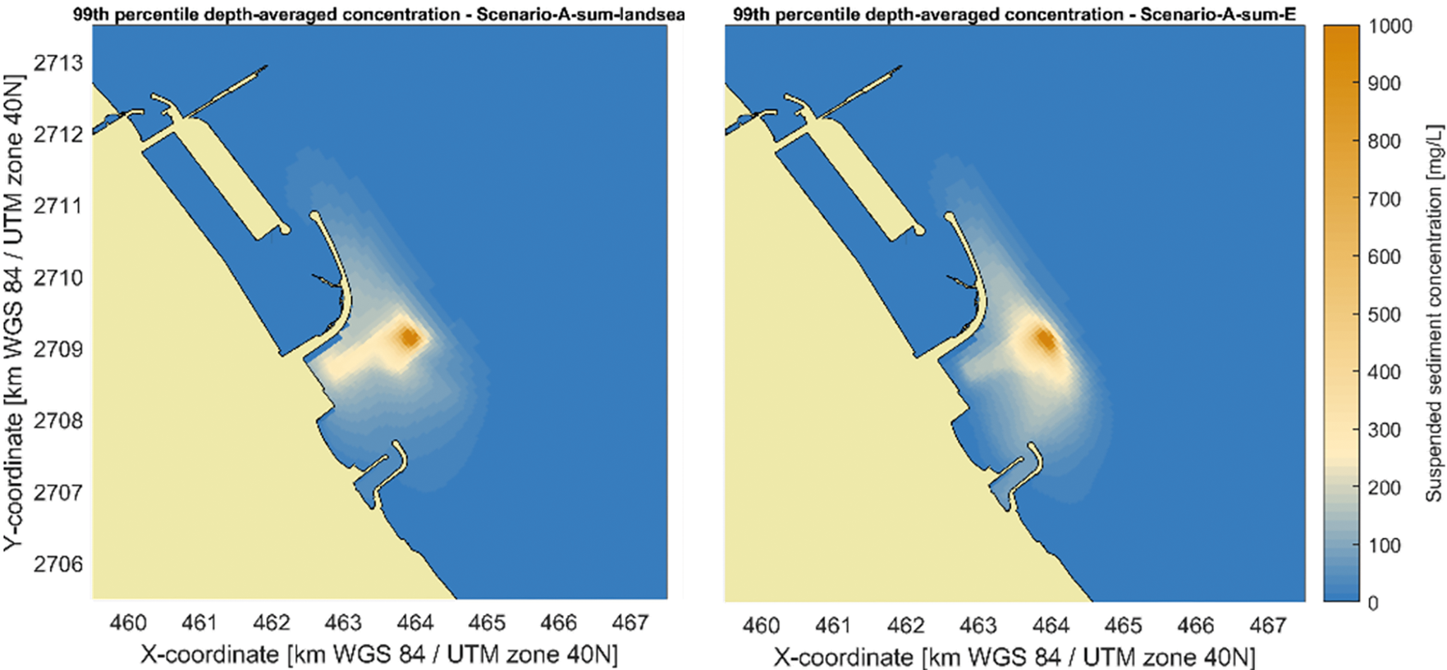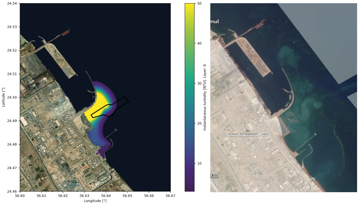In Figure 2, the model outcome is presented for maximum (99th percentile) depth- averaged suspended sediment concentration (SSC) for the typical land-sea breeze and the more severe Eastern wind during the summer.

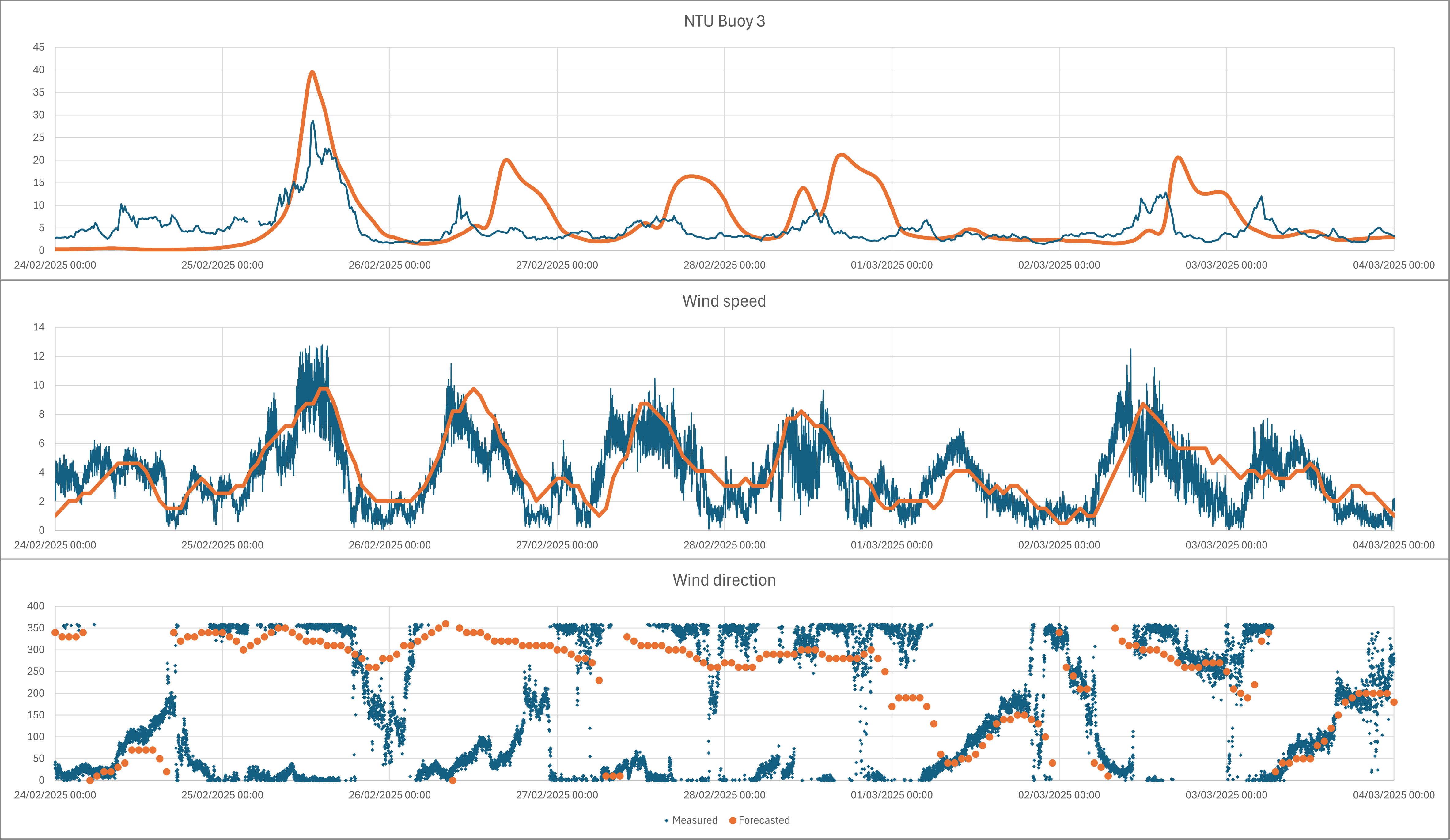
Each scenario is modeled independently, but in reality combinations of operations with different equipment and methods may occur, particularly in projects with ambitious timelines. These factors highlight the importance of adopting an adaptive dredging method, one that is based on real-time monitoring and forecasting. This approach allows for the optimisation of dredging operations while minimising environmental impact.

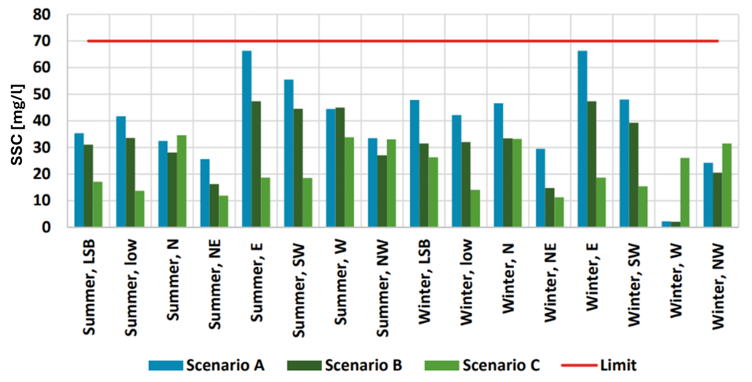
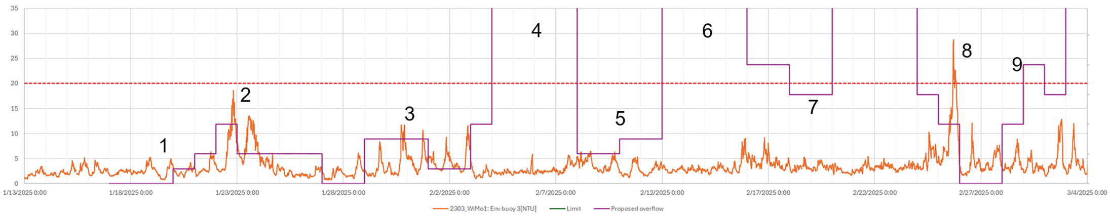
The outcome of the modelling exercise is presented in Figure 3. It shows the maximum computed excess suspended sediment concentration over the simulation period at the intake location for the different scenarios considered. The highest values experienced do not exceed 70 mg/l (equal to approx. 20 NTU) and are related to dredging scenario under Eastern wind conditions. Further, the dredging operations as modelled in Scenario C (no overflow) clearly show lower values across most of the different wind conditions, which can be helpful as a turbidity control mitigation measure.

The modelling assessment also highlighted that, under certain unfavorable ambient conditions the turbidity value of 20 NTU for the seawater intake could be exceeded because the background turbidity is not included in the model. The same was discussed with stakeholders in order to obtain the relevant permits and NOC's and to set turbidity limits for the project. Turbidity limits must both prevent disturbance of the seawater intake and enable an economically feasible dredging project. The outcome of the pre-tender modelling (as presented in Figure 3) was helpful for the authorities to define the allowable turbidity limits for the project in the permits.

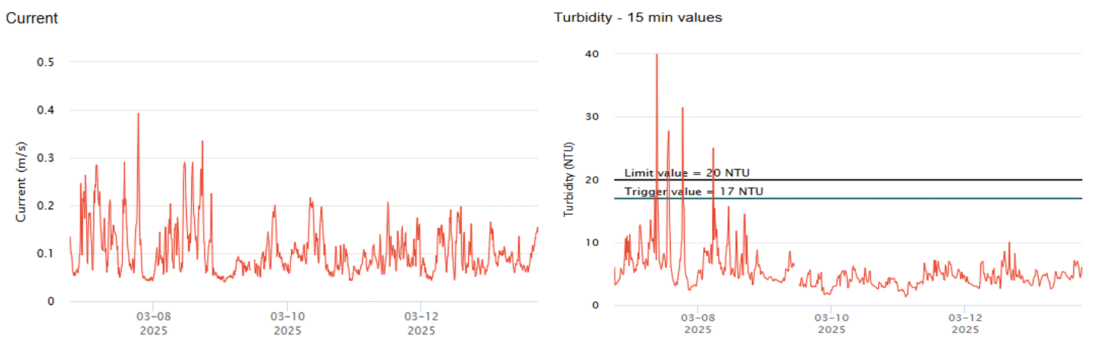
Following the turbidity assessment and Environmental Impact Assessment, a permit was granted by the seawater intake operator for the dredging activities incorporating strict turbidity limits. The not-to-exceed turbidity limits (including background value), as defined, are:

• Maximum allowed weekly average of 15 NTU; and
• Maximum allowed peak turbidity of 20 NTU for no more than a period of 15 minutes in one hour.

Tender and execution turbidity plume modelling

After the tender process, the project was awarded to Boskalis. The turbidity challenge transferred from the tender stage through to the successful completion of the project. Pre-tender turbidity studies rely on general information on dredging vessels and their source terms, which are crucial for a project to progress to execution. For dredging contractors, these studies provide a foundation to work from, but the assumptions need calibration and modification to develop project-specific work methods. Sharing information from the models developed during the pre-tender stage significantly enhances the contractor's ability to implement tailored work methods that benefit the project.

Turbidity model application during tender stage

For the project, Boskalis recreated a Delft3D Flexible Mesh (Delft3D-FM) model. Model assumptions from the pre-tender modelling assessment by Deltares were adopted, such as:

• Fall velocity of fine soil fractions.
• Model extents.
• Tidal boundary conditions.
• Wind scenarios.
• NTU to mg/l relationship.
• Average weather conditions.

Assumptions on the source terms were re-evaluated based on the source term assumptions of (Becker, 2015) and IADC (Laboyrie, 2018). Using the work methods and production estimates from the tender stage, the recreated model was utilised to estimate the impact of turbidity during operations. Average weather statistics estimated during the pre-tender phase were employed to identify the most stringent scenarios that required adaptation to prevent exceeding the intake NTU limits.

Operations causing turbidity

The work method planned during the tender stage involved dredging the majority of the material with a trailing suction hopper dredger (TSHD). An existing hard layer required the use of a backhoe dredger (BHD) to remove the material. The primary causes of turbidity include both the drag head and overflow of the TSHD.

Dredging with the BHD, filling barges, and ploughing activities were expected to have a much smaller impact compared to the TSHD and were therefore not considered to be governing. Depending on the soil conditions, the source terms were calculated using Becker's methodology (Becker, 2015), resulting in the source terms provided in Table 1. These source terms are significantly lower compared to the pre-tender estimated source terms, which were too conservative. The numbers indicate the effect of a shorter overflow time when dredging in sand. Dredging silt was assumed to be carried out without overflow, as overflow losses were expected to be large; however, due to the abundance of fines, the source term was expected to remain high. The source term for dredging rock was expected to be limited due to lower production rates and the trapped fines within the rock.

Operational measures for turbidity control

The highest contributor to the source term is the overflow from the TSHDs. This factor can be easily adjusted to mitigate turbidity in adverse weather conditions. Consequently, the decision was made to allow for lower production by limiting the overflow time in situations where the weather necessitates it. Table 2 shows the turbidity plume modelling conducted for various weather scenarios. By combining the percentage of occurrence for each weather scenario, a total overflow reduction has been determined for the project.

Pre-defined dredging scenarios listed in Table 3 have been modelled with wind scenarios. This results in an expected reduction in the source term. If a reduction of the source terms is required, adaptive management must be applied by reducing the overflow time of the TSHDs.

In total, it is expected that the NTU limits will be exceeded during 15% of the project duration if no adaptive management is applied, assuming a 3 NTU background turbidity and based on unrestricted overflow times. The goal of proactive adaptive management during project execution is to mitigate these exceedances and remain within the NTU limits.

Due to the critical turbidity levels significantly affecting the production rates of the vessels, a proactive adaptive management dredging approach, as proposed by CEDA (CEDA, 2024), has been developed for implementation during the execution phase.

Automated turbidity model development and use during execution

During the execution of the project, average occurrences of weather events are no longer valuable because they do not provide the necessary details for immediate decision- making and risk management. Instead, accurate weather predictions and associated mitigation measures are required for the foreseeable future. This requires additional sources of information, including:

• Water level forecasts;
• Wind forecasts;
• Production forecasts; and
• Intake volume forecasts for the seawater intake.

Of this list, the water level forecast is relatively straightforward, as the water levels are primarily caused by the tide, which can be predicted for any moment in time using tidal constituents. The wind forecast, being the main driver of the currents, is procured from expert weather forecasters. The production forecast is made internally based on optimal desired overflow times to achieve maximum production in a dredging cycle. Fluctuations in intake volumes and potential forecasts have been investigated; however, due to a lack of information and seemingly stable intake volumes, this factor was kept constant throughout the project.

To automatically run the Delft3D FM+WAQ model on a daily basis, the Microsoft Azure platform (Microsoft, n.d.) was utilised. Containerised processes and an in-house developed orchestrator perform multiple tasks either in sequence or simultaneously, in a so-called model train. This model train, in simplified form, can be schematised as shown in Figure 4. The input data is automatically downloaded via API calls or from internal network locations. Following this, the data is processed into suitable Delft3D input files for the hydrodynamic model. The production forecast is then used to calculate source terms for the Delft3D WAQ model. The outcomes of this run are automatically analysed against the NTU limits specified by the project. If the unmitigated results indicate an exceedance of the limits, the source terms are adjusted accordingly and the WAQ model is restarted. Model results are post-processed; hourly spatial plots are generated, and data is exported into graphs for use in a forecast dashboard. The output from the mitigated WAQ model run after one day is used as the input for the model run on the following day. As the plume remains suspended for 1 to 3 days, cumulative errors are short-lived and can be addressed by calibrating the model.

This final step of reusing model output for the next day's model run is crucial because the history of the plume is a significant factor in estimating the impact of turbidity. Depending on the settling velocity of the fine material, sediment plumes can remain in suspension for hours or even days. Therefore, the turbidity plume from the previous day can greatly influence the following day's concentration results; hence, the model should start with an existing plume each day.

Automated daily forecasting based on dredging and weather forecast

Since wind prediction is the main uncertainty among the environmental drivers of the model and the prediction becomes less reliable further into the future, it is important to limit the amount of time the model forecasts. However, because the impact of dredging on measured turbidity has a time lag of hours to days, it is essential to model at least the lifespan of the plume. In other words, the source term at moment A will influence the measurement at moment B. To mitigate a potential exceedance at moment B, the source term at moment A must be lowered. To provide flexibility in how far the model needs to forecast, three days are modelled. This means that, in total, the model will look 4 to 5 days into the future, depending on when the model is initiated.

Since the weather forecast can become less reliable over such time frames, the interval between starting a model and implementing its results must be as short as possible. If a model were 100% reliable, this period could be limited to the model runtime. However, because model results can be uncertain, additional time is reserved for interpretation and rerunning if necessary. Daily reanalysis of the forward-looking window is performed to minimize wind forecast uncertainty. The model timings are schematized in Figure 5.

Pro-active adaptive dredging approach

When the model results become available, they will be interpreted. This interpretation is crucial because the model is an approximation of reality. Therefore, the interpretation must consider the differences and their potential implications. Examples of differences between the model and reality include:

• Variability in weather predictions or deviations in measured conditions;
• Re-suspension or reduced settling velocities due to wave action not accounted for in the model;
• Variations in dredging productions;
• Equipment breakdowns;
• Changes in soil conditions;
• Alterations in dredging locations; and
• Updates to bathymetry.

Once the interpretation has been completed, mitigation measures can be determined. The primary mitigation measure is adjusting the overflow time, but the dredging location is often also considered when critical situations arise. Mitigation measures can be implemented on a day-to-day basis or immediately in response to rapid changes in weather conditions.

Continuous turbidity monitoring

Continuous live turbidity monitoring with buoys has been implemented for multiple reasons:

• To show contractual compliance to the NTU limitations;
• To check model results versus reality;
• To act as an early warning system in case the model results are deemed unreliable;
• To measure background turbidity in the event of natural high turbidity events; and
• To measure other important parameters, such as chlorophyll, dissolved oxygen and current speeds.

The measurement buoys' locations are shown in Figure 6.

Buoy 1 and buoy 4 are designated as background buoys, buoy 2 serves as the early warning buoy and buoy 3 along with the quay wall station are buoys used to demonstrate compliance with contractual limits. Buoy measurements started prior to project execution for a baseline study on the background turbidity values. During project execution additionally spatial handheld NTU profiles over depth are measured multiple times per week at fixed locations within the dredging area for model calibration and validation. Figure 7 shows an example of handheld turbidity readings on the measurement grid. These handheld measurements provide valuable information to verify the concentrations in the forecasted plume and indicate the level of conservatism. If modelled levels are deemed too conservative, a manual calibration of forecasted NTU levels is performed. Handheld readings generally show lower values within 500 metres of the dredging area, which can be explained by the conservative settling velocity used in the model, accounting for the reduced settling caused by propeller wash.

Stakeholder involvement

The live buoy measurements are shared with relevant stakeholders through an online dashboard. Additionally, stakeholders are informed about the daily turbidity model and its interpretation. A daily turbidity forecast report is distributed, which includes the general outcomes of the model runs, the interpretation and its consequences on the mitigation measures.

Implementation and validation

During the initial stages of the project, a soft start to the dredging activities was implemented to account for assumptions in the model and to build confidence in the model results. During this ramp-up period, the model was calibrated by taking soil samples, analysing satellite imagery and conducting NTU measurements. After the ramp-up period, the conservativeness of the initial model was reduced by lowering the overflow source term fraction with a factor 2, linearly impacting the SSC in the plume. The forecasted production rates and dredging cycle times are adjusted to better reflect actual conditions.

Periodic validation and model update with on-site measured data

As the project progressed, both the soil and bathymetry changed. When it was determined that these changes significantly altered model outcomes, a model update was implemented. This was deemed necessary after approximately 50% of the project was completed and harder soil had been dredged. The harder soil required longer overflow times due to less efficient dredging. However, this did not necessarily lead to a higher average source term since the percentage of fines was lower and the fines were trapped in lumps of material.

As the project progresses and parameters change, deciding whether to update the interpretation or the model can be challenging. Updating the interpretation works well in the short term, but postponing a model update can result in the model becoming increasingly divergent from reality. However, updating the model comes with the downside that the interpretation of the model may change again. To address this, a test and a production model train are run separately. Model updates are first implemented in the test environment. When the test results are deemed reliable and the differences with the main production model train are understood, the model train is updated. This approach helps avoid errors in running the model train or in the interpretation.

Results and discussion

Accuracy of turbidity forecasting model

An example of model output from 25 February to 3 March is shown in Figure 8. This event is used to illustrate how the model functions and why the interpretation phase is important. Trends in the plume are predicted relatively well. The graphs show examples of events where the model predicted high turbidity and the measurements also showed spikes. The timing and level of turbidity events occasionally is inaccurate, which can be explained by differences in:

• The actual vs. modelled dredging cycle: A theoretical dredging cycle is implemented in the forecast model, which is unlikely to align exactly with the real dredging cycle. It is challenging to predict the exact timings when a vessel is dredging.
• The actual vs. modelled overflow times: Predicted overflow times are implemented in the model; however, real overflow times may differ due to varying soil types.
• The actual vs. modelled wind conditions: Predicted wind conditions often show differences from measured wind conditions. Variations in directions and peak velocities influence the currents in the model.
• Wave conditions, which are not included in the model.

The predicted turbidity levels during the peaks are overestimated by the model. This is due to a conservative settling velocity chosen to account for the increased turbulence caused by propeller wash. The low ambient velocities are significantly influenced by propeller wash eddies over larger distances, which cannot be captured in the Delft3D model. The effect of this can be clearly seen in current velocity peaks in buoy 2, which coincide with turbidity peaks, as shown in Figure 9. The spikes around 8 March align with the turbidity spikes. The effect of vessel movement can also be observed when comparing satellite imagery with model output in Figure 10. Local eddies with high concentrations can be seen, whereas the model predicts a much more gradual plume. The plume location aligns well, although local differences due to vessel movements are visible. Satellite or drone imagery proved to be a valuable tool to verify model results during the interpretation phase.

Impact on project execution

Taking the interpretation after the model results into account, advice is provided on which mitigation measures can be applied to remain within the limits. These measures may include options beyond overflow reduction, such as:

• Dredging in deeper water to prevent propeller wash;
• Avoiding dredging high up on the slopes of the design to prevent propeller wash;
• Choosing to dredge in a different material with lower fines content with overflow;
• Opting to dredge in a location with many fines without overflow; and
• Scheduling repairs or bunkering of one of the vessels to lower the total source term of the project.

Figure 11 shows the indicative proposed overflow duration against the buoy 3 turbidity readings and the turbidity limit of 20 NTU. This figure demonstrates how effective the overall approach of the model train with an interpretation phase has been for the project. Events where overflow time was restricted could have resulted in exceedances of the limit if no mitigating measures had been implemented. Conversely, during periods with low turbidity risks and thus no restrictions, the measurements show low turbidity values and optimal overflow times for maximum production were implemented. Several noteworthy events are listed in Figure 11.

From the above, it is concluded that although the predictive modelling shows some uncertainty, it provides significant confidence as a method for making decisions during project execution. Changes in weather systems are generally well captured and the general idea of the turbidity risk is known a few days in advance. The uncertainty of the model predictions will decrease over time as measured data provides information to update the model or the interpretation of the model results. The exact turbidity level will remain difficult to model precisely since local disturbances, such as eddies from vessel propellers, cannot be captured in a predictive model. This uncertainty will persist throughout the project and therefore must be considered when advising on mitigation measures.

Challenges and lessons learned

Model validation before project execution

When the project started, the model was not calibrated and validated due to the absence of measured data during dredging activities. A comparison was made with the pre-tender turbidity assessment, which showed similar results. Validation and calibration of the model was required at the beginning of the project. During this phase, communication with stakeholders regarding the model's performance was essential to maintain trust in the model train.

Field data of soil is lagging behind on model forecasts

Soil samples from the hopper are taken and analysed continuously. The process time between taking a sample and receiving its results should be as short as possible, as dredging is ongoing and soil can change. For smaller projects, the soil data may not be fully representative for updating model settings if soil conditions change quickly with dredging depth. Sampling must be done carefully to ensure it provides a comprehensive picture of the dredged material.

Propeller wash turbidity

Separating turbidity caused by propeller wash from that generated by the drag head and overflow is challenging. In shallow areas, propeller wash is likely to be a significant source term. This is assumed to be accounted for by additional conservatism in the dredging source term.

Vessel movement

Effects from the vessel propellers appear to influence the current patterns in and near the dredging area. Buoy 2 indicated that spikes in current velocity significantly reduced during bunkering or repairs. Additionally, satellite imagery consistently showed a pattern in the plume, with an inflow of clear water into the dredging area from where the vessels started sailing towards the disposal area and old eddy-shaped plumes towards the south and north. With the current models, it is not feasible to include a moving propeller wash forcing, which means this factor must be considered during the interpretation phase after the model run.

Wave impact

Waves appeared to have a significant impact on (background) turbidity during periods of increased wave height. This was observed once during the baseline measurements and twice during dredging when no exceedance was predicted by the model. Waves were not included in the model as they were expected to be of low importance. Despite this, the majority of the time, waves did not have a substantial impact. Unforeseen effects during periods of increased wave height were considered during the interpretation phase of the model results.

CONCLUSION

Summary of findings

• A turbidity forecast model is an effective tool for determining short-term dredging strategies, considering the impact of predicted weather on sensitive receivers such as a seawater intake.
• Uncertainties in the turbidity forecast can be managed by the contractor. There are various mitigation measures beyond adjusting overflow duration, such as dredging in different locations, deeper water, different materials and planning repairs.
• Adaptation of the model compared to reality always lags behind real-time data. When soil conditions change, this leads to additional uncertainty. The source term is highly dependent on soil type and overflow duration alone as a mitigation measure can be a poor indicator when transitioning to a different material type. System knowledge is critical and the contractor can assess experience from the project and measurements to estimate the risk.
• As the project progresses and parameters change, deciding whether to update the interpretation or the model can be challenging. Updating the interpretation is easier in the short term, but postponing the model update for too long can cause the model to deviate significantly from reality.
• Satellite or drone imagery can greatly assist in calibrating and validating the model. The shape and intensity of the historical plume generated by previous dredging are crucial for accurate model results but are very difficult to verify with local measurements only.
• Investing in proper communication with stakeholders builds mutual trust. Online dashboards and visualisations are highly valuable tools for this purpose.
• The execution phase validated many pre- tender conclusions but also highlighted the need for ongoing adjustments based on real-time data. Continuous monitoring and adaptive management proved essential for maintaining environmental compliance and optimising productivity.

Significance of the forecasting model and adaptive approach

For the Sohar Port development project, the forecast model proved to be a valuable tool for making operational decisions. Applying a pro-active adaptive dredging strategy based on forecasted predictions led to reduced environmental impact and improved dredging and overall project performance, meeting the requirements set by stakeholders.

Recommendations for future projects

• A thorough system understanding backed by measurements during the pre-tender phase greatly increases the possibility of reliable and valuable forecast modeling for the project.
• Due to intrinsic uncertainty in turbidity forecasting, implementing realistic limits that can be exceeded for an acceptable duration helps to reduce an overly conservative approach. This includes allowances for spikes in turbidity readings that cannot be captured by a forecast model.
• Turbidity management is most beneficial if implemented by the contractor. This provides flexibility in the mitigation measures and benefits the project by allowing the trade-off between risk and production, considering all nuances known by the contractor. Providing reliable and sufficient site data by the client during the tender phase is crucial for an accurate risk assessment.
• Making the turbidity models used during the pre-tender stage available during the tender stage greatly enhances the contractor's flexibility to implement specific work methods, benefiting the project overall.
• Engage stakeholders regularly for open communication and share insights from models and forecasts.